Felipe Gonzalez Web Page Programas/Diffusion Equation

Programas

Diffusion Equation

The diffusion equation allows to describe the dynamics of a diffusive system, such as the temperature in a material, the movement of ink in water, and even the propagation of cancer cells in the brain. In the following, we will show some applications of this equation:

$\frac{\partial\phi(\mathbf{r},t)}{\partial t} = \nabla \cdot \big[ D(\phi,\mathbf{r}) \nabla\phi(\mathbf{r},t) \big].$

EXAMPLES

1D Diffusion Equation: cooling a rod from both ends
Tumor growth model

1D Diffusion Equation

The simplest problem where the diffusion equation appears is in the hear flux along a one dimensional rod of length $L$ , subjected to the boundary conditions $T(0,t)=T_1$ y $T(L,t)=T_2$ , where $T(x,t)$ is the temperature at a distance $x$ from the left edge at a time $t$ . If the diffusion coefficient is constant (the bar is homogeneous), then we can write the diffusion equation as

$\frac{\partial T(x,t)}{\partial t} = D\, \nabla^2 T(x,t),$

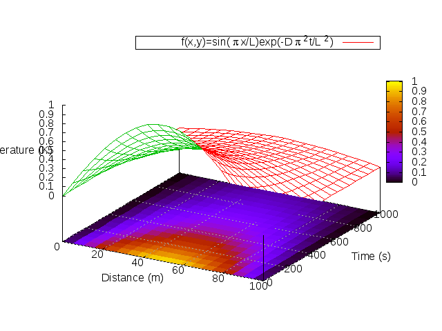
where $D$ is the diffusion coefficient that characterizes the material from which the rod is made of. For the particular case in which we keep the edges cold ( $T(0,t)=0$ , $T(L,t)=0$ ) and an initial profile $T(x,0)=\sin(\pi x/L)$ , the problem can be solved analytically, and the solution is

$T(x,t) = \sin\left(\frac{\pi x}{L}\right)\exp\left(-\frac{D \pi^2 t}{L^2}\right).$

We can solve the diffusion equation numerically through finite differences, using the FTCS scheme:

$\frac{T_j^{n+1}-T_j^n}{\Delta t}=D\frac{T_{j+1}^n-2T_j^n+T_{j-1}^n}{(\Delta x)^2},$

that we can write as

$T_j^{n+1}=T_j^n+D\,r(T_{j+1}^n-2T_{j}^n+\,T_{j-1}^n),$ ,

where $T_j^n=T(x_j,t_n)$ is the temperature in the position $x_j=j \Delta x$ at the time $t_n=n\Delta t$ , and $r=\Delta t/(\Delta x)^2$ . Here, $\Delta x=L/(N-1)$ is the size of the $N$ divisions (from $0$ to $N-1$ ) of the interval $\left[0,L\right]$ , such that $x_0=0$ and $x_{N-1}=L$ ; while $\Delta t$ is the time step, which must fulfill the numerical convergence criteria

$2D\Delta t \leq \Delta x^2$ .

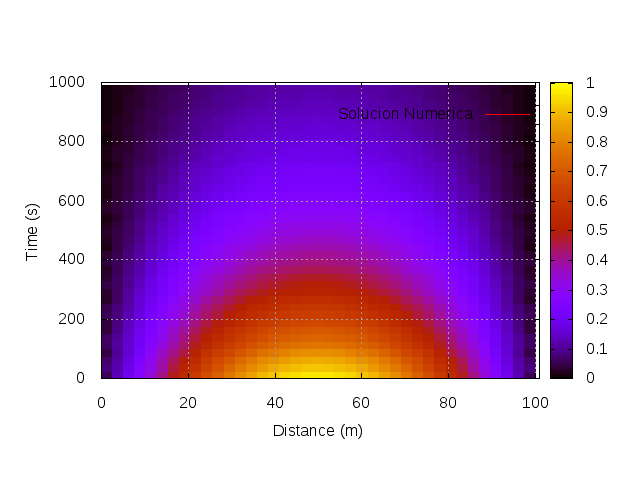
In this way, we can get to the same analytical solution and then solve more complicated problems for this system, which don't have analytical solution. We now show the analytical solution versus the numerical solution:

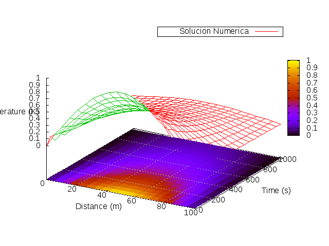Código (C++)

#include<iostream>
#include<fstream>
#include<cmath>
using namespace std;

//const double D=2.2;
const int Ndx=70, tmax=1000; // segundos
const double L=100.0; // metros
const double Tmax=5; // Kelvin
const double dx=L/(Ndx-1), dt=0.9*(dx*dx/(2.0*3.2)), r=dt/(dx*dx);

// Coeficiente de difusion
double D(double x)
{
// double Dx = (x<L/2.0)? 3.2 : 0.2; // metros²/segundo
double Dx = 2.2;
return Dx;
}

// Condicion de Borde 1: T(0,t)=g1(t)
//double g1(double t){ return 1+500*exp(-0.001*(t-100)*(t-100));}
//double g1(double t){ return 1+(Tmax-1)*(2*atan(t/100)/M_PI);}
double g1(double t){ return 0.0;}
// Condicion de Borde 2: T(L,t)=g2(t)
double g2(double t){ return 0.0;}
// Condicion Inicial: T(x,0)=f(x) (Se debe cumplir f(0)=T(0,0)=g1(0) y f(L)=T(L,0)=g2(0))
double f(double x){ return sin(M_PI*x/L);}

int main()
{
double T[Ndx]; // T(x,t)
double Tant[Ndx]; // T(x,t) (copia)
for (int j=0; j<Ndx; j++) T[j]=0;

// Condicion inical
for (int j=0; j<Ndx-1; j++) T[j]=f(j*dx);

ofstream arch("calor.dat");
arch << "#x" << "\t" << "#t" << "\t" << "T(x,t)" << endl;

for (double t=0; t<=tmax; t+=dt)
{
if (int(t/dt)%50==0)
{
/* DIBUJO GNUPLOT */
cout<<"plot [0:"<<L<<"][0:" << Tmax << "]";
cout << " '-' w l ls 3 lw 8 t 'D=3.2',"; // Puntos para la barra
cout << " '-' w l ls 2 lw 8 t 'D=1.2',"; // Puntos para la barra
cout << " '-' ls 2 lc 0 t 'Time: t=" << t << "'" << endl; // Puntos T(x,t)
cout << "0 0" << endl << L/2 << " 0" << endl; // La barra va de (0,0) a (L/2,0)
cout << 'e' << endl; // Terminamos los 2 puntos que definen la barra.
cout << L/2 << " 0" << endl << L << " 0" << endl; // La barra va de (0,0) a (L/2,0)
cout << 'e' << endl; // Terminamos los 2 puntos que definen la barra.
for (int j=0; j<Ndx; j++)
{
arch << j*dx << " " << t << " " << T[j] << endl;
cout << j*dx << " " << T[j] << endl;
}
cout << 'e' << endl << flush;
}
// Aplicando condiciones de Borde
T[0]=g1(t);
T[Ndx-1]=g2(t);
// Haciendo una copia del arreglo
for(int j=0; j<Ndx; j++) Tant[j]=T[j];
// Resolviendo entre medio
for (int j=1; j<Ndx-1; j++)
{
T[j]=Tant[j] + D(j*dx)*r*(Tant[j+1]-2*Tant[j]+Tant[j-1]);
}
}
cout << "pause 2" << endl;
arch.close();
return 0;
}

[$[Get Code]]

Compilado el programa, ejecutar con

./programa | gnuplot

[$[Get Code]]

Código (python)

from pylab import *
from numpy import *
Ndx=70; tmax=50; # segundos
L=100.0; # metros
Tmax=5.0; # Kelvin
D=20.0
dx=L/(Ndx-1); dt=0.8*(dx*dx/(2.0*D)); r=dt/(dx*dx)
Temp = []

# Condicion de Borde 1: T(0,t)=g1(t)
def g1(t): return 0.0
# Condicion de Borde 2: T(L,t)=g2(t)
def g2(t): return 0.0
# Condicion Inicial: T(x,0)=f(x) (Se debe cumplir f(0)=T(0,0)=g1(0) y f(L)=T(L,0)=g2(0))
def f(x): return Tmax*sin(pi*x/L);

T = [0.0]*Ndx # T(x,t)
Tant = [0.0]*Ndx # T(x,t) (copia)
# Condicion inical
for j in xrange(Ndx-1): T[j]=f(j*dx)
#print "#x","#t","#T(x,t)"

for n in xrange(int(tmax/dt)):
# Aplicando condiciones de Borde
t=n*dt
T[0]=g1(t)
T[Ndx-1]=g2(t)
# Haciendo una copia del arreglo
Tant=list(T)
# Resolviendo entre medio
for j in xrange(Ndx-1):
T[j]=Tant[j] + D*r*(Tant[j+1]-2*Tant[j]+Tant[j-1])

# Cada 10 pasos...
if (int(t/dt)%10==0):
# Anadimos al arreglo de temperaturas la lista de temperaturas en este paso
Temp += [ list(T) ]
# for j in xrange(Ndx):
# print j*dx, t, T[j]
Temp = array(Temp)

from mpl_toolkits.mplot3d.axes3d import get_test_data
fig = plt.figure()
ax = fig.add_subplot(1, 1, 1, projection='3d')
X = array([j*dx for j in xrange(Ndx)] )
Y = array([n*dt for n in xrange(len(Temp))] )
X, Y = meshgrid(X, Y)
Z = Temp
surf = ax.plot_surface(X, Y, Z, rstride=1, cstride=1, cmap=cm.coolwarm, vmin=0, vmax=Tmax, linewidth=0, antialiased=False)
ax.set_zlim3d(0, Tmax)

show()

[$[Get Code]]

Modelo de crecimiento de un tumor

Existen varios modelos que permiten estudiar el crecimiento de un tumor. Uno de los modelos más simples para modelar la evolución de un glioblastoma en presencia de quimioterapia se puede formular postulando que la tasa de crecimiento de células cancerígenas tiene un término difusivo y uno de crecimiento poblacional, es decir,

$\frac{\partial c}{\partial t} = \nabla\cdot (D \nabla c) + \rho c - G(t)c,$

donde $c=c(\vec r, t)$ es la concentración de células tumorales en un sitio $\vec r$ en un tiempo $t$ , y $G(t)$ es una función que describe los efectos de la quimioterapia. El coeficiente de difusión $D$ en general depende de la concentración de células cancerígenas $c$ , es decir, $D=D(c(\vec r,t))$ .

Si suponemos simetría esférica, podemos expresar la ecuación anterior como

$\frac{\partial c}{\partial t}$

$=$

$\frac{\partial D}{\partial r}+\frac{\partial D}{\partial c}\frac{\partial c}{\partial r}$

$+$

$D(c)\left(\frac{\partial^2 c}{\partial r^2}+\frac{1}{r}\frac{\partial c}{\partial r}\right) + \rho c - G(t)c$

Para este caso particular, vamos a elegir

$D(c)=D_{min}+ \frac{2}{\pi}(D_{max}-D_{min})\arctan(c)$ ,

de modo que $D=D_{min}$ en zonas donde $c=0$ , y vale a lo más $D_{max}$ cuando la concentración es muy grande. Resolvemos la ecuación usando diferencias finitas, tal como suele resolverse la ecuación de difusión.

Para comenzar, daremos una condición inicial correspondiente a un tumor localizado en el centro del cerebro, como muestran las figuras a continuación.

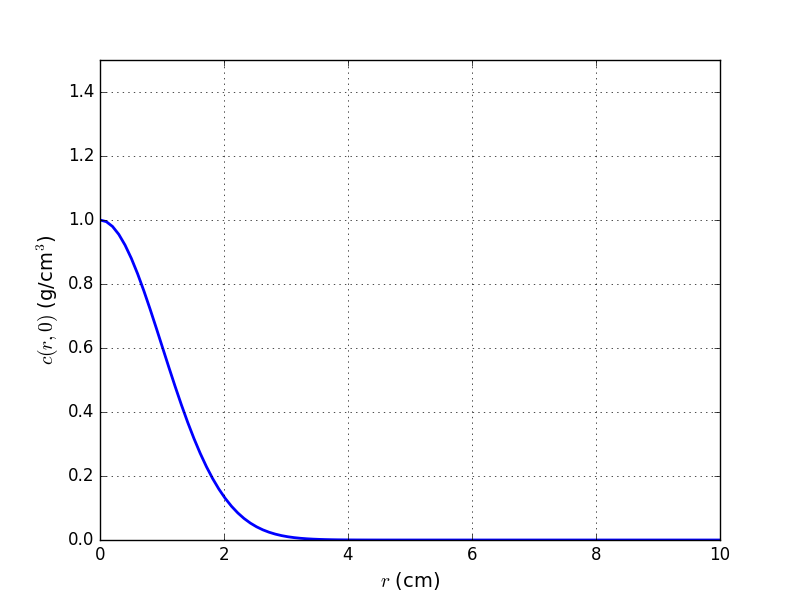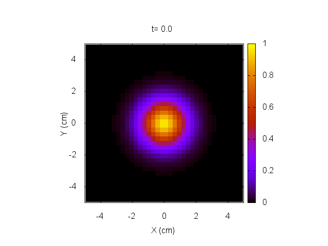Usando un tratamiento representado por dos pulsos a los 200 y 500 segundos, dados por

$G(t) = 10\rho\exp\left(-\frac{(t-200)^2}{1000}\right)+10\rho\exp\left(-\frac{(t-500)^2}{1000}\right)$

hacemos evolucionar el sistema y lo mostramos a continuación.

En este caso, el tratamiento $G(t)$ no es capaz de eliminar el tumor, el cual sigue creciendo sin control.

Código (python)

#***********************************************************************#
#* ECUACION DE CRECIMIENTO DE UN TUMOR CEREBRAL *#
#* *#
#* Este programa encuentra la solucion a una de las ecuaciones *#
#* propuestas para la propagacion de un tumor, tomada del *#
#* trabajo de Tiberiu Harko y M. K. Mak: *#
#* TRAVELLING WAVE SOLUTIONS OF THE REACTION-DIFFUSION MATHEMATICAL *#
#* MODEL OF GLIOBLASTOMA GROWTH: AN ABEL EQUATION BASED APPROACH: *#
#* dc/dt = V.(D Vc) + rho*c - G(t)c *#
#* donde c=c(r,t) es la densidad de celulas tumorales en la *#
#* posicion r en tiempo t, rho la tasa neta de proliferacion, *#
#* y D=D(c(r)), el coef. de difusion, que depende de c. *#
#* G(t) es una funcion de influencia externa, que representa el *#
#* efecto de la quimioterapia. *#
#* *#
#* Suponiendo simetria radial, se obtiene *#
#* dc/dt = D'(c(r))*(dc/dr)^2 + D(c(r))*d^2c/dr^2 + rho*c - G(t)c *#
#***********************************************************************#
# AUTOR: FELIPE GONZALEZ CATALDO, Octubre 2015.

from numpy import *
R=9.9 # Radio del cerebro (cm)
N=100 # Divisiones del intervalo [0,R]
Dmax=0.010 # Maximo coeficiente de difusion (ver D abajo), en cm^2/sec
Dmin=0.001 # Minimo coeficiente de difusion (ver D abajo), en cm^2/sec
rho=0.005 # rho= tasa neta de proliferacion, en 1/sec
dr=R/(N-1)
dt=0.8*dr*dr/(2*Dmax) # Mientras mas grande la difusion, mas chico debe ser dt
t=0.0; tmax=2000.0
c = [0.0]*N
c_ant = [0.0]*N

# Coeficiente de difusion:
def D(c,r):
return Dmin+ 0.63661977*(Dmax-Dmin)*arctan(c) # 2/pi=0.6366

# Derivada parcial del coef. de difusion respecto a c (derivar arriba):
def Dc(c,r):
return 0.63661977*(Dmax-Dmin)/(1+c*c)

# Derivada parcial del coef. de difusion respecto a r (derivar arriba):
def Dr(c,r):
return 0.0

# Condicion inicial c(r,0)=f(r)
def f(r):
return exp(-50*(r/R)**2) if r<R/2.0 else 0.0

# When chemotherapy is administered, G(t) is constant, and G(t) = 0 otherwise
def G(t):
return 10*rho*exp(-(t-200)**2/1000)+10*rho*exp(-(t-500)**2/1000) #+100*rho*exp(-(t-2000)**2/1000)

def PrintForGnuplot(u):
# Con esta funcion imprimimos la funcion para gnuplot: r, c(r)
print "plot [0:",R,"][0:5] '-' w l ls 12 lw 3 title 't=", t,"'"
for j in xrange(N):
print j*dr, c[j]
print "end"
print "set grid"
# print "pause",1

def PrintContoursGnuplot(u):
# Con esta funcion imprimimos un mapa de contornos pm3d map de gnuplot
# print "set isosample 10,10"
print "set dgrid3d 31,31,31"
print "set pm3d map"
print "set cbrange [0:1]"
print "set title 't=", t,"'"
print "splot [-"+str(R)+":"+str(R)+"][-"+str(R)+":"+str(R)+"][] '-' title 't=", t,"'"
No = 15
do = 2.0*pi/No
for i in xrange(No):
for j in xrange(N):
x=j*dr*cos(i*do);
y=j*dr*sin(i*do);
print x, y , c[j]
print "e"
# print "set grid"

# Condicion inicial c(r,0)=f(r)
for j in xrange(N):
c[j]=f(j*dr);
c_ant[j]=f(j*dr);

interval = int(tmax/dt/500)
while(t<=tmax):
# if int(t/dt)%interval==0: PrintForGnuplot(c)
if int(t/dt)%(interval*20)==0: PrintContoursGnuplot(c)

#*** METODO PREDICTOR ****#
# Primero los bordes
c[0] = c_ant[0] + dt*( D(c_ant[0],0*dr)*(4.0*(c_ant[1]-c_ant[0])/(dr*dr)) )
c[0] += dt*( rho*c_ant[0] - G(t)*c_ant[0] )
c[N-1]=0.0 # c(R)=0
# Luego entre medio
for j in xrange(1,N-1):
dcdr = (c_ant[j+1]-c_ant[j-1])/(2.0*dr)
c[j] = c_ant[j] + dt*( dcdr*( Dr(c_ant[j],j*dr) + Dc(c_ant[j],j*dr)*dcdr ) )
c[j] += dt*( D(c_ant[j],j*dr)*(c_ant[j+1]-2*c_ant[j]+c_ant[j-1])/(dr*dr) )
c[j] += dt*( D(c_ant[j],j*dr)*dcdr/(j*dr) )
c[j] += dt*( rho*c_ant[j] - G(t)*c_ant[j] )
#************************#
# Guardamos las posiciones nuevas para la vuelta siguiente
c_ant = list(c)
t+=dt
# >>END OF WHILE<<

[$[Get Code]]

« Programs

Felipe Gonzalez Web Page

Diffusion Equation

Código (C++)

Código (python)

Código (python)

Search

Options: