Ising Model
The Ising model is a mathematical model that allows to study a system of interacting spins (or magnetic dipoles). The model in 2 dimensions predicts a phase transition at low temperature, where the system becomes magnetized. The system is modelled by the Hamiltonian
The spin-spin interaction is classified as follows:
: ferromagnetic
: antiferromagnetic
: non-interacting
According to the analytical solution, found by Lars Onsager, the phase transition takes place at a critical temperature
for the isotropic case (). The average magnetization is given, in the Onsager solution, by
EXAMPLES
| No External Magnetic Field |
|---|
The simplest version of the Ising model considers only first neighbors interaction, and no external magnetic field. The Hamiltonian in this case is
where is the same for all spin pair interactions.
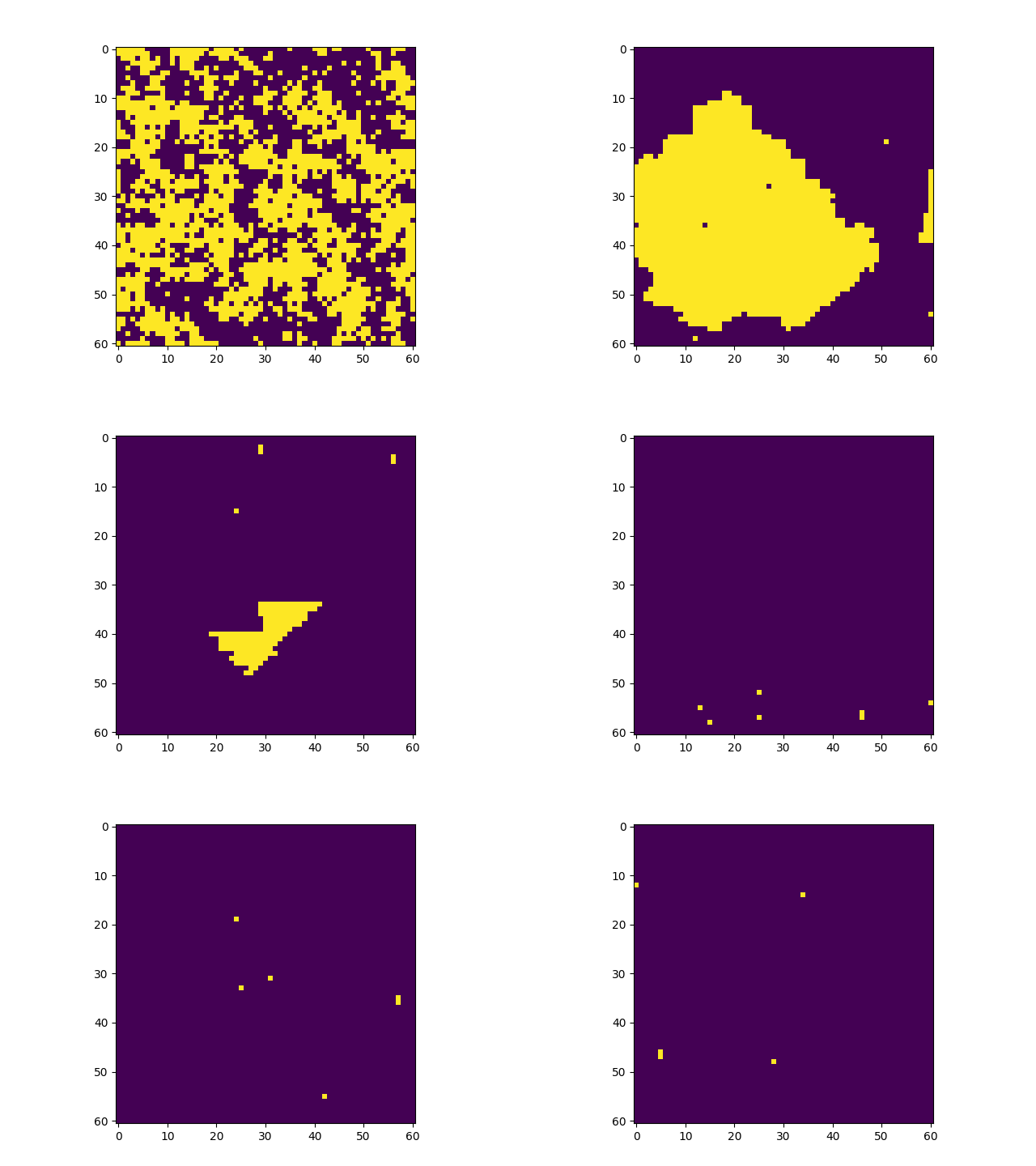
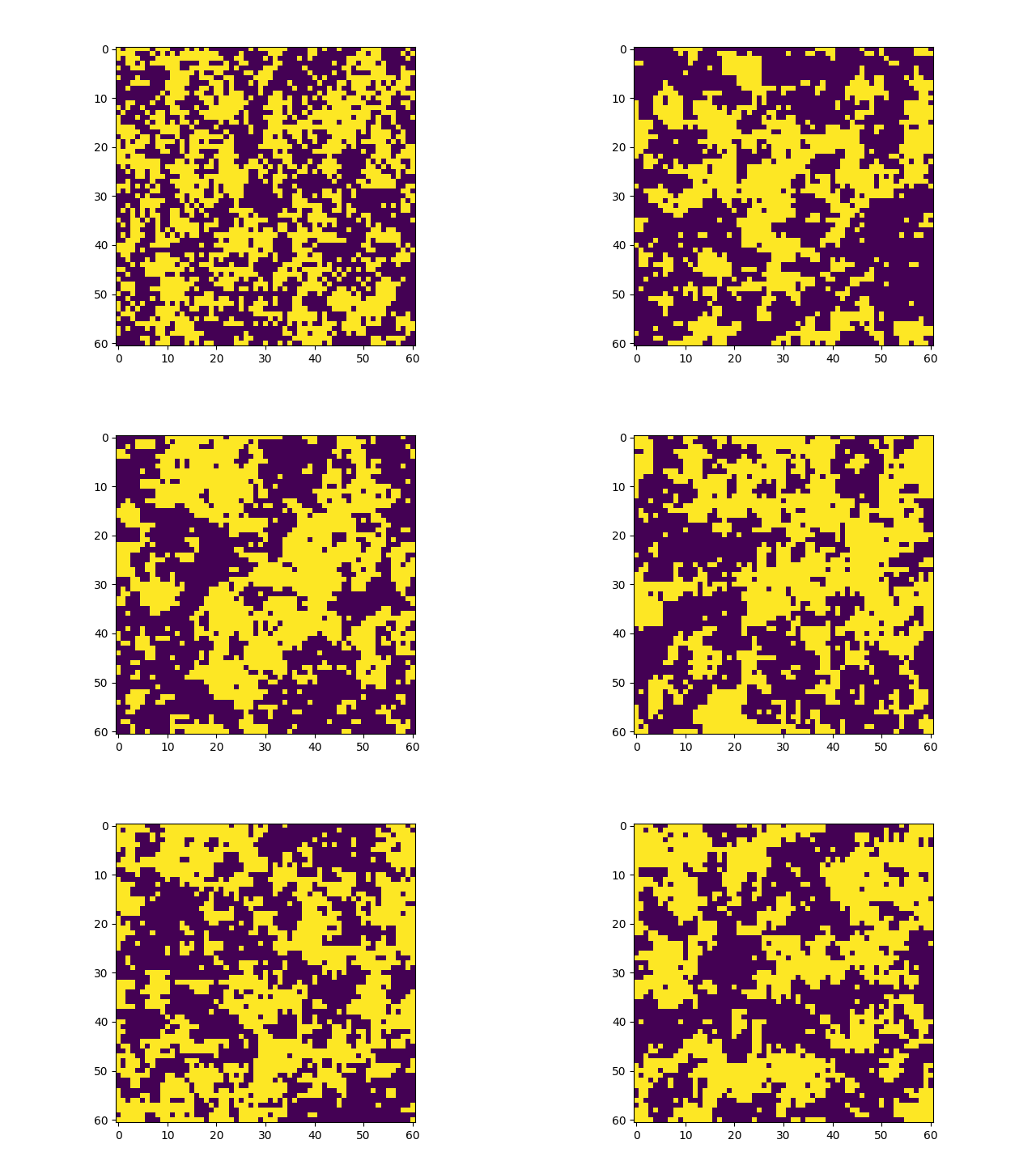
The system is initialized in a random configuration of +1 and (-1) and evolves according to the Metropolis-Hasting algorithm. In just a few steps, the system becomes magnetized. | |
The temperature is higher than the transition temperature. There is no phase transition, the system does not get magnetized. | |
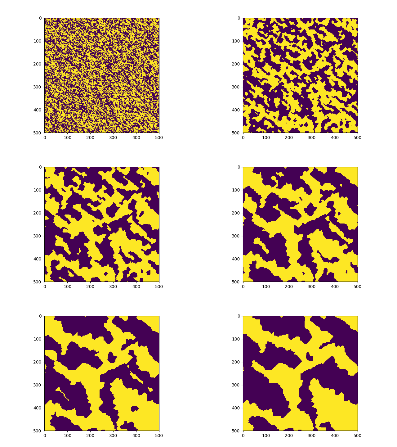
Phase transition in a larger system (500x500). |
Code (python)
#***********************************************************************#
#* THE ISING MODEL *#
#* *#
#* This program uses the Metropolis Monte Carlo algorithm *#
#* to simulate the Ising model, with Hamiltonian *#
#* ---- *#
#* H = \ -J_ij * Si*Sj *#
#* / *#
#* ----ij *#
#* *#
#* Adapted from B. Militzer course, EPS109, UC Berkeley, 2018. *#
#***********************************************************************#
# AUTHOR: FELIPE GONZALEZ CATALDO, September 2018.
from pylab import *
fig = figure(1)
ax = subplot(111)
# Jij = J for all i,j: Coupling constant (Jij>0: ferromagnetic, Jij<0: antiferromagnetic, Jij=0: non magnetic )
J= 1 # In eV, ferromagnetic
kT = 1.2*J # In eV
# ONSAGER SOLUTION FOR 2D LATTICE: kT = 2*J/(ln(1+sqrt(2))) = 2.2691853
n=61
mat = random(size=(n,n)) # Matrix of randoms in the interval [ 0.0 1.0 ]
mat = 2*floor(2*mat)-1 # Martrix of random 1's and -1's
img = imshow(mat)
show(block=False)
nBlocks = 100
for iBlock in xrange(nBlocks):
for ix in xrange(n):
ixp = (ix+1) % n # Neighbor to the right
ixm = (ix-1) % n # Neighbor to the left
for iy in xrange(n):
iyp = (iy+1) % n # Neighbor above
iym = (iy-1) % n # Neighbor below
s = mat[ixm,iy] + mat[ixp,iy] + mat[ix,iyp] + mat[ix,iym] # Sum of neighbors spins
mOld = mat[ix,iy] # Old value of the spin
EOld = -J*mOld*s # Si * (S_above + S_below + S_left + S_right)
mNew = -mOld
ENew = -J*mNew*s # sum_ij Si'*Sj, where Si' = -Si
Ediff = ENew - EOld # No need to sum over all the lattice, just this (ix,iy) site energy.
prob = exp(-Ediff/kT)
if ENew < EOld:
mat[ix,iy] = mNew
else:
mat[ix,iy] = mNew if random() < exp(-Ediff/kT) else mOld
#print iBlock
img.set_data(mat)
plt.pause(1e-30)
draw()
#savefig('is'+str(iBlock)+'.png')

